Diagnosing Video Stuttering Over TCP: A JitterTrap Investigation

Your security camera feed stutters. Your video call over the corporate VPN freezes. The question isn’t whether something is wrong—that’s obvious. The question is what is wrong, because the fix depends entirely on the diagnosis.

Is the problem the sender, the network, or the receiver? These require fundamentally different interventions. Telling someone to “upgrade their internet connection” when the real issue is their overloaded NVR is worse than useless—it wastes time and money while the actual problem persists.

Sender-side problems—where the source isn’t transmitting at the expected rate—are straightforward to detect: compare actual throughput to expected throughput. The harder question is distinguishing network problems from receiver problems when data is being sent. TCP’s built-in feedback mechanisms give us the answer.

UDP is the natural transport for real-time video—it tolerates loss gracefully and avoids head-of-line blocking. But video often ends up traveling over TCP whether we like it or not. VPN tunnels may encapsulate everything in TCP. Security cameras fall back to RTSP interleaved mode (RTP-over-TCP) when UDP is blocked. Some equipment simply doesn’t offer a choice.

The research question driving this investigation: Can we identify reliable TCP metrics that distinguish network problems from receiver problems?

Through controlled experiments, I found the answer is yes—with important caveats. This post builds a complete diagnostic framework covering all three problem types, with the experiments focused on the harder network-vs-receiver distinction. Part 2 will explore what happens when TCP goes chaotic.

---

TCP Flow Control: Two Feedback Mechanisms

Before we can diagnose problems, we need to understand what TCP is actually doing when video stutters. TCP provides two distinct feedback mechanisms, and confusing them is the source of most misdiagnosis.

What TCP Guarantees

TCP exists to provide reliable, ordered byte streams over an unreliable network. It achieves this through:

1. Sequence numbers: Every byte gets a number; the receiver can detect missing data
2. Acknowledgments: The receiver confirms what it has received
3. Retransmission: The sender resends anything that goes missing
4. Flow control: The receiver can slow down the sender
5. Congestion control: The sender adapts to network capacity

The last two are critical for diagnosis, and they’re often conflated. Let me be precise about what each one does.

Flow Control: The Receiver’s Brake Pedal

Flow control is the receiver saying “slow down, I can’t keep up.” Here’s how it works:

Every TCP segment the receiver sends back includes a window advertisement—a number representing how many bytes of buffer space remain available. The sender is not allowed to have more unacknowledged data in flight than this window permits.

When the receiver’s buffer fills up (because the application isn’t reading fast enough), the advertised window shrinks. If it reaches zero, TCP sends a zero-window notification. The sender must stop transmitting until the receiver advertises space again.

Zero-window events are the receiver explicitly telling the sender: “I’m overwhelmed.” This is unambiguous. If you see zero-window advertisements, the receiver has a problem.

Congestion Control: The Network’s Speed Limit

Congestion control is the sender’s attempt to discover network capacity without overwhelming it. Unlike flow control, this is typically implicit—the sender infers congestion from indirect signals rather than explicit messages.

The traditional signal is packet loss. When packets go missing (detected by timeouts or duplicate acknowledgments), TCP interprets this as congestion and reduces its sending rate. This triggers retransmissions—the sender resends the lost data. Packet loss is consistent, measurable, and actionable, which is why loss-based congestion control dominates.

Some algorithms take a different approach. BBR, for instance, monitors RTT (Round-Trip Time)—the time for a packet to reach the receiver and for the acknowledgment to return. When router queues fill, RTT increases before packets actually drop. By detecting this early signal, BBR can respond to congestion before loss occurs.

ECN (Explicit Congestion Notification) offers another alternative: instead of dropping packets, ECN-capable routers mark them with a CE (Congestion Experienced) bit. The receiver echoes this back via the ECE (ECN-Echo) flag in TCP, and the sender acknowledges with CWR (Congestion Window Reduced). This provides explicit congestion signaling without the cost of packet loss.

Retransmits generally indicate that packets were lost in transit. The causes vary—congestion, faulty links, wireless interference—but they all represent network-layer problems rather than receiver-layer problems. (Spurious retransmits from packet reordering can occur, but in aggregate, elevated retransmit counts reliably signal network issues.)

The Key Insight

These mechanisms give us observable signals:

Signal	What It Means	Where the Problem Is
Zero-window events	Receiver buffer filled	Receiver
Retransmissions	Packets lost in transit	Network
ECN-Echo (ECE) flags	Router signaled congestion	Network (queue filling)

This seems straightforward. If you see zero-window events, it’s a receiver problem. If you see retransmits, it’s a network problem. But ECN adds valuable nuance: it can distinguish queue congestion (routers filling up) from random packet loss (wireless interference, cable issues). The reality is more nuanced, as we’ll see, but this is the foundation.

---

Observing TCP Signals in Practice

Before presenting experimental results, let me show you how to observe these signals yourself. This matters because claims about TCP behavior should be verifiable.

Counting Zero-Window Events with tshark

The tcp.analysis.zero_window filter catches zero-window advertisements:

# Count zero-window events in a capture
tshark -r capture.pcap -Y "tcp.analysis.zero_window" | wc -l

# Watch for zero-window events in real-time on interface eth0
tshark -i eth0 -Y "tcp.analysis.zero_window" -T fields \
    -e frame.time_relative -e ip.src -e ip.dst -e tcp.window_size

What does a healthy stream look like? In a well-functioning video stream, you should see zero or very few zero-window events. When I see more than 5 in a 10-second window, something is wrong with the receiver.

Counting Retransmissions with tshark

For retransmits, use tcp.analysis.retransmission:

# Count retransmissions in a capture
tshark -r capture.pcap -Y "tcp.analysis.retransmission" | wc -l

# Watch for retransmits in real-time
tshark -i eth0 -Y "tcp.analysis.retransmission" -T fields \
    -e frame.time_relative -e ip.src -e ip.dst -e tcp.seq

In a healthy network, retransmits should be rare—perhaps a handful over minutes. When I see more than 10 retransmits in 10 seconds, that indicates significant packet loss.

Counting ECN-Echo (ECE) Flags with tshark

ECE flags indicate explicit congestion notification from routers:

# Count ECE flags in a capture
tshark -r capture.pcap -Y "tcp.flags.ece == 1" | wc -l

# Watch for ECE flags in real-time
tshark -i eth0 -Y "tcp.flags.ece == 1" -T fields \
    -e frame.time_relative -e ip.src -e ip.dst

ECE flags only appear when both endpoints negotiate ECN support and a router marks packets with the CE (Congestion Experienced) bit. When I see more than 2 ECE flags in 10 seconds, that indicates queue congestion somewhere in the path.

A Practical Diagnostic Script

Here’s a script that implements a simplified version of the diagnostic hierarchy. It uses throughput comparison for sender detection (rather than inter-packet gap measurement, which requires per-packet timing analysis). For on-demand capture and analysis:

#!/bin/bash
# tcp-diag.sh - TCP diagnostic following the framework hierarchy
# Usage: tcp-diag.sh [interface] [duration] [expected_mbps]

IFACE="${1:-eth0}"
DURATION="${2:-10}"
EXPECTED_MBPS="${3:-}"  # Optional: expected throughput in Mbps

echo "Capturing on $IFACE for $DURATION seconds..."
tshark -i "$IFACE" -a duration:"$DURATION" -w /tmp/diag.pcap 2>/dev/null

# Gather metrics
ZERO_WIN=$(tshark -r /tmp/diag.pcap -Y "tcp.analysis.zero_window" 2>/dev/null | wc -l)
RETRANS=$(tshark -r /tmp/diag.pcap -Y "tcp.analysis.retransmission" 2>/dev/null | wc -l)
ECE=$(tshark -r /tmp/diag.pcap -Y "tcp.flags.ece == 1" 2>/dev/null | wc -l)
BYTES=$(tshark -r /tmp/diag.pcap -T fields -e frame.len 2>/dev/null | awk '{s+=$1} END {print s+0}')
ACTUAL_MBPS=$(echo "scale=2; $BYTES * 8 / $DURATION / 1000000" | bc)

echo "Results over $DURATION seconds:"
echo "  Throughput: ${ACTUAL_MBPS} Mbps"
echo "  Zero-window events: $ZERO_WIN"
echo "  Retransmissions: $RETRANS"
echo "  ECE flags: $ECE"
echo ""

# Diagnostic hierarchy (order matters!)
TCP_HEALTHY=$(( ZERO_WIN <= 5 && RETRANS <= 10 ))

# 1. SENDER CHECK: Low throughput with healthy TCP signals?
if [ -n "$EXPECTED_MBPS" ]; then
    THRESHOLD=$(echo "$EXPECTED_MBPS * 0.5" | bc)  # 50% of expected
    LOW_THROUGHPUT=$(echo "$ACTUAL_MBPS < $THRESHOLD" | bc -l)
    if [ "$LOW_THROUGHPUT" -eq 1 ] && [ "$TCP_HEALTHY" -eq 1 ]; then
        echo ">> SENDER PROBLEM: ${ACTUAL_MBPS} Mbps vs ${EXPECTED_MBPS} Mbps expected"
        echo "   TCP signals healthy - sender not transmitting enough data"
        rm /tmp/diag.pcap; exit 0
    fi
fi

# 2. RECEIVER CHECK: Zero-window events?
if [ "$ZERO_WIN" -gt 5 ]; then
    echo ">> RECEIVER PROBLEM: $ZERO_WIN zero-window events"
    echo "   Network must be OK (otherwise masking would hide this)"
    rm /tmp/diag.pcap; exit 0
fi

# 3. NETWORK CHECK: Retransmissions?
if [ "$RETRANS" -gt 10 ]; then
    echo ">> NETWORK PROBLEM: $RETRANS retransmissions"
    # 4. Refine with ECE
    if [ "$ECE" -gt 2 ]; then
        echo "   ECE flags present - queue congestion + packet loss"
    else
        echo "   No ECE - random packet loss (check link quality)"
    fi
    echo "   WARNING: Receiver status unknown (may be masked) - re-test after fix"
    rm /tmp/diag.pcap; exit 0
fi

# Check for pure congestion (ECE without retransmits)
if [ "$ECE" -gt 2 ]; then
    echo ">> QUEUE CONGESTION: $ECE ECE flags, but no packet loss yet"
    echo "   Router signaling 'slow down' - reduce bitrate"
    rm /tmp/diag.pcap; exit 0
fi

echo ">> HEALTHY: No significant problems detected"
rm /tmp/diag.pcap

With the theory understood and observation tools in hand, let’s look at what the experiments revealed.

---

The Diagnostic Framework

The goal of this investigation was to develop a practical diagnostic framework for stuttering TCP streams—and to determine whether JitterTrap could be useful in applying it. To do that, I needed to reproduce the common pathologies (network congestion, packet loss, receiver overload) in a controlled environment where I could verify the ground truth.

I ran controlled experiments using network namespace isolation and tc/netem for precise impairment injection. Each experiment simulated a specific failure mode with known parameters, then measured whether TCP’s observable signals correctly identified the cause.

The Test Topology

The bridge namespace allows precise control of delay, jitter, and loss using tc netem. The receiver can be configured to stall (simulating CPU load) to create receiver-side problems.

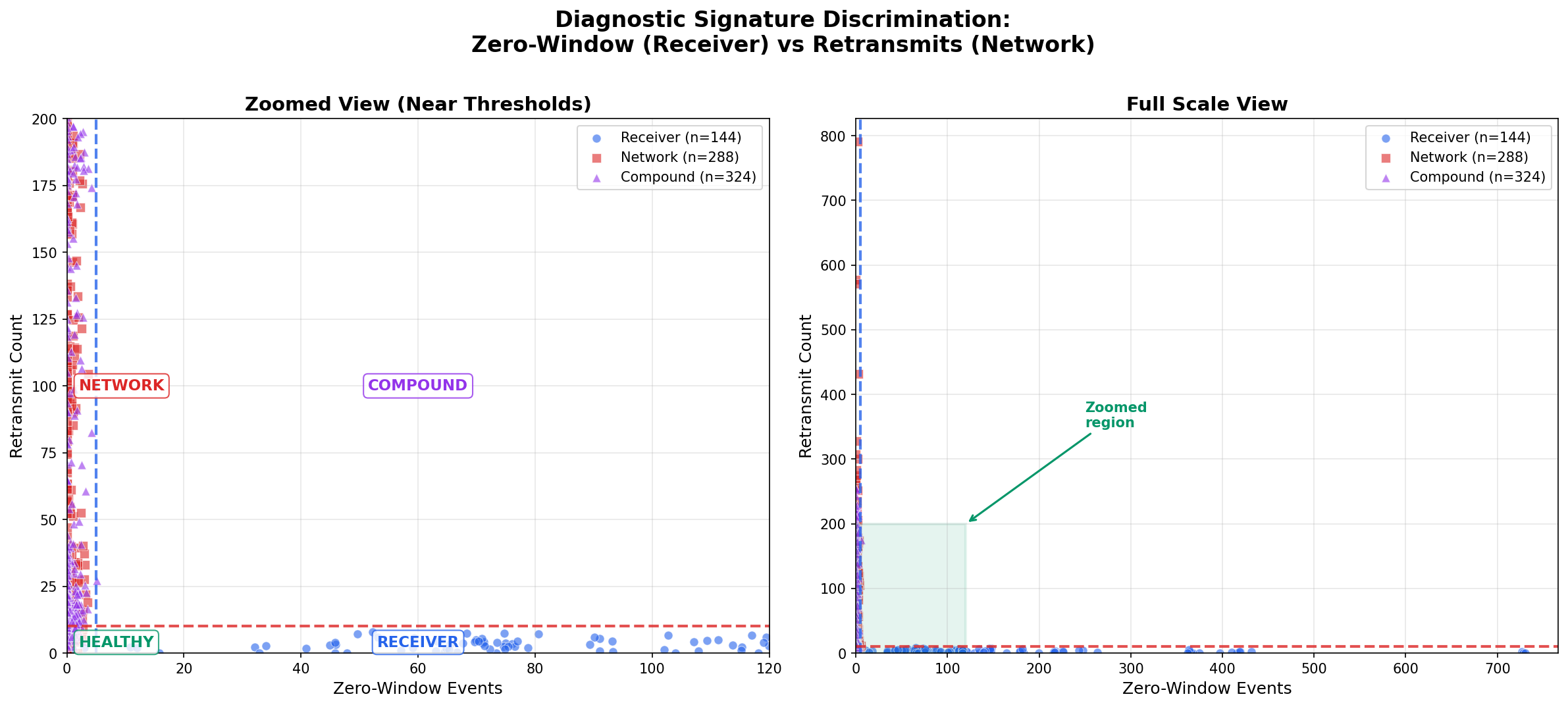
Three Experiment Categories

The experiments tested three scenarios:

1. Pure receiver problems: Network is clean; receiver experiences CPU stalls of 10-100ms
2. Pure network problems: Receiver is fast; network has jitter, delay, or loss
3. Compound problems: Both receiver stalls and network impairment present

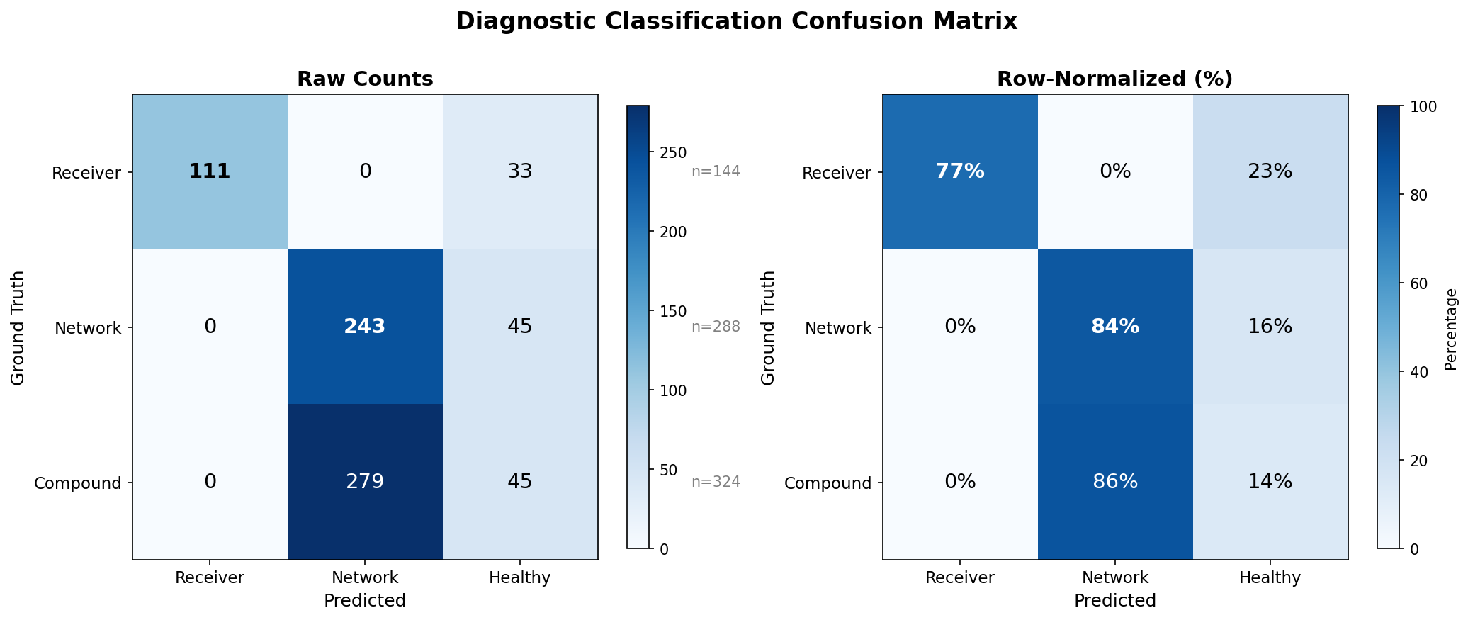
Results: The Signatures Work

Problem Type	Zero-Window > 5	Retransmits > 10	Correct Classification
Pure Receiver	77%	5%	77%
Pure Network	0%	84%	84%
Compound	0%	87%	Network detected, receiver masked

The discrimination is good but not perfect:

• 77% accuracy for receiver problems: Some mild stalls don’t produce enough zero-window events to cross the threshold
• 84% accuracy for network problems: Some mild impairments don’t cause enough retransmits to cross the threshold
• 5% false positive for receiver: Even with a clean network, severe receiver stalls can trigger retransmits—TCP’s persist timer probes during zero-window conditions are sometimes classified as retransmissions by packet analyzers
• Compound problems: The network problem was correctly detected (87% showed retransmits > 10), but zero-window events never appeared—the receiver problem was invisible

A note on thresholds: The values used here (>5 zero-window events, >10 retransmits, in 10 seconds) are empirical heuristics tuned against this experimental data. They represent a reasonable trade-off between sensitivity and specificity for the conditions tested. Your environment may require different thresholds—the principle (count these events, compare to a threshold) matters more than the specific numbers.

That last row demands explanation.

---

The Masking Effect: A Fundamental Limitation

The most important finding from this research isn’t a number—it’s a qualitative discovery about how TCP behaves under compound problems.

Network Problems Hide Receiver Problems

When both network impairment and receiver stalls are present, zero-window events disappear entirely. Every compound experiment showed zero zero-window events, even when the receiver was configured to stall.

Why? TCP’s congestion control is too good.

When the network is impaired (causing retransmits), the TCP stack detects loss and congestion control algorithms like CUBIC respond by throttling the sender. The sender slows down so much that data never arrives faster than the slow receiver can process it. The receiver’s buffer never fills. Zero-window is never advertised.

The receiver problem is masked by the network problem.

The Diagnostic Implication

This has a profound implication for diagnosis:

If You See	Diagnosis	What It Tells You
Zero-window > 5	Receiver problem	Network is OK (otherwise masking would hide this)
Retransmits > 10, no zero-window	Network problem	Receiver status unknown (could be masked)
Neither	Healthy, or problems below threshold	—

When you detect a network problem, you cannot determine whether the receiver also has a problem. The network problem must be fixed first. Then you can re-test to check for receiver issues.

Conversely, if you see zero-window events, the network is functioning well enough to deliver data faster than the receiver can process it. A severely impaired network would throttle the sender, preventing receiver overload.

This isn’t a flaw in the diagnostic method—it’s a fundamental property of TCP flow control. The masking effect is real and unavoidable.

---

Refining Network Diagnosis: Congestion vs Random Loss

You’ve identified a network problem—retransmits exceed the threshold. But retransmits only tell you packets were lost, not why. The next question matters because the fixes differ:

• Queue congestion (router buffers filling): Reduce bitrate, the path can’t sustain this rate
• Random loss (wireless interference, cable faults): Investigate the physical layer, the path itself is degraded

This is where ECN proves its value. Recall that ECN-capable routers mark packets with CE bits when queues fill, and receivers echo this back via ECE flags. The key insight: ECE flags indicate queue-based congestion, while retransmits without ECE suggest random loss.

ECN Findings

Scenario	ECE > 2	Retransmits > 10	Correct Classification
Congestion only	Yes	No	100%
Random loss only	No	Yes	97%
Mixed (both)	Yes	Yes	71%

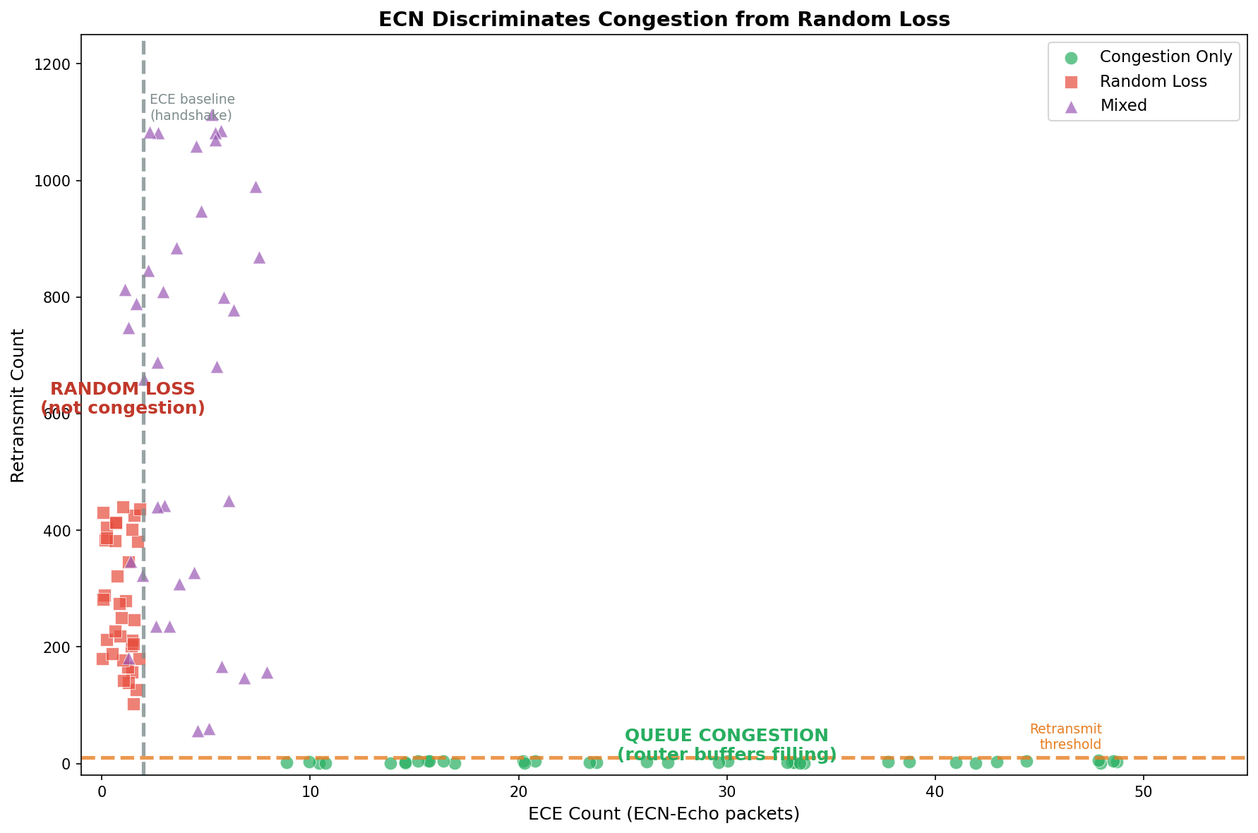
The scatter plot shows clear separation: queue congestion (green circles) clusters at low retransmits with elevated ECE counts, while packet loss (red squares) clusters at high retransmits with only baseline ECE from the TCP handshake. The dashed lines show our diagnostic thresholds.

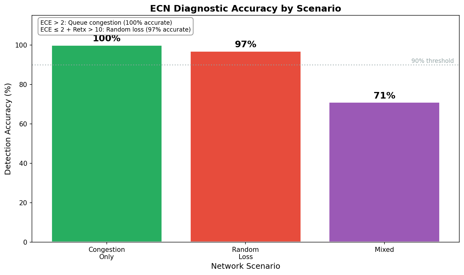
ECN successfully distinguishes congestion from random loss with high accuracy in single-cause scenarios. Mixed scenarios are harder—but knowing both problems exist is still valuable.

The Complete Diagnostic Hierarchy

The experiments above focused on receiver and network problems. Additional experiments validated sender problem detection using inter-packet gap (IPG) analysis.

When a sender stutters, it manifests as gaps between packets—periods where no packets are sent at all. Unlike network congestion (packets queued or lost) or receiver problems (window throttling), sender problems show up as large inter-packet gaps with healthy TCP indicators. Across 134 sender-stall experiments:

• 100% had zero zero-window events (the receiver isn’t overwhelmed—it’s simply not receiving data)
• IPG closely matches stall duration (a 500ms stall produces a ~500ms gap, R² > 0.99)
• 94.4% classification accuracy using the threshold: IPG > 60ms with healthy TCP signals

Why 60ms? This threshold isn’t universal—it’s tuned for 30fps video. At 30fps, each frame spans ~33ms. A 60ms gap means at least one frame was delayed or dropped—visible as a stutter. The threshold should match your application:

Application	Frame/Update Rate	Suggested IPG Threshold
Real-time gaming	60fps (16ms)	> 20-30ms
Interactive video	30fps (33ms)	> 50-60ms
Buffered streaming	Variable	> 100-200ms (buffer-dependent)
Surveillance/NVR	15fps (66ms)	> 100ms

The threshold must also exceed the path RTT to distinguish sender stalls from normal ACK-clocked pacing. The refined formula: IPG > max(application_threshold, RTT × 1.2).

Bringing together all three problem types:

Check	Observable	Threshold	Diagnosis
1. Inter-packet gaps	Time between packets	Application-dependent (e.g., > 60ms for 30fps video)	Sender problem
2. Zero-window	Receiver window advertisements	> 5 events / 10s	Receiver overload (network must be OK)
3. Retransmits	Lost packet recovery	> 10 events / 10s	Network problem (receiver status unknown)
4. ECE flags	Explicit congestion signals	> 2 events / 10s	Refines network: queue vs random loss

The order matters:

1. Inter-packet gap check first: Large gaps (>60ms) with no zero-window and no retransmits indicate the sender isn’t transmitting. Problem is upstream.

2. Zero-window second: If present, the receiver can’t keep up—and we know the network is OK (otherwise masking would hide this).

3. Retransmits third: Indicate network problems. When present, receiver status is unknown due to masking. Fix network first, then re-test.

4. ECE last: Refines network diagnosis between queue congestion and random loss.

RTT ceiling limitation: Sender stalls are only detectable when the stall duration exceeds the RTT. TCP’s ACK-clocked pacing naturally creates inter-packet gaps proportional to RTT, so a 100ms stall on a 100ms RTT path looks like normal pacing. The refined threshold is: IPG > max(application_threshold, RTT × 1.2).

Caveats

ECN requires end-to-end support. Both endpoints and all routers in the path must have ECN enabled. Many networks don’t—in which case you’ll see zero ECE flags regardless of actual congestion. Absence of ECE doesn’t prove absence of congestion; it may just mean ECN isn’t deployed.

ECE without retransmits is pure congestion. The router signaled “slow down” before dropping packets. This is actually the best-case network problem—early warning before loss occurs.

---

What JitterTrap Already Does

The diagnostic script above works for post-hoc analysis, but it requires capturing traffic at the right moment—which means knowing when problems will occur. JitterTrap solves this by providing real-time analysis and continuous capture. You can monitor flows live and trigger captures when anomalies appear, without predicting when stuttering will happen.

JitterTrap provides the raw observables for this diagnostic framework—but not yet the automated diagnosis. Following the diagnostic hierarchy, let’s look at how JitterTrap supports each check.

Sender Detection: Throughput and Top Talkers

The first diagnostic check compares actual throughput to expected throughput. JitterTrap’s throughput view shows an oscilloscope-inspired real-time display of bitrate and packet rates. If your camera should be streaming at 4 Mbps but you’re seeing 500 Kbps with healthy TCP indicators, the problem is upstream—likely the sender itself.

The top talkers view helps identify which flows are underperforming. Combined with Traps (threshold-based packet capture that triggers when rates drop below expected levels), you can catch sender stuttering patterns as they happen.

JitterTrap’s Inter-Packet Gap chart directly measures the time between consecutive packets—the key metric for detecting sender stalls.

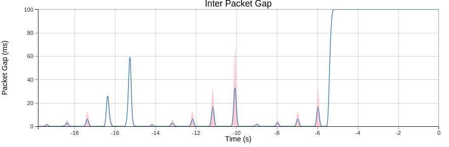
This capture demonstrates sender stall characterization using an increasing stall pattern: 5ms, 10ms, 20ms, 50ms, and 100ms pauses, repeated multiple times. The first two repetitions are fully visible; the third is partially clipped as the 100ms stall coincides with the end of the test. Despite the clipping, the pattern clearly shows what different stall durations look like—essential during product development when you need to verify that your encoder, transcoder, or application maintains consistent packet timing under various loads.

Notice the distinct spikes at different heights. The smaller stalls (5-20ms) produce small spikes, the ~60ms spike sits right at the video threshold boundary, and the 100ms stall produces a clear plateau. For 30fps video, only stalls above ~60ms would trigger a “sender problem” alert—but for 60fps gaming (20-30ms threshold), even the 25ms stalls would be flagged.

The corresponding throughput view shows the same pattern as dips in bitrate:

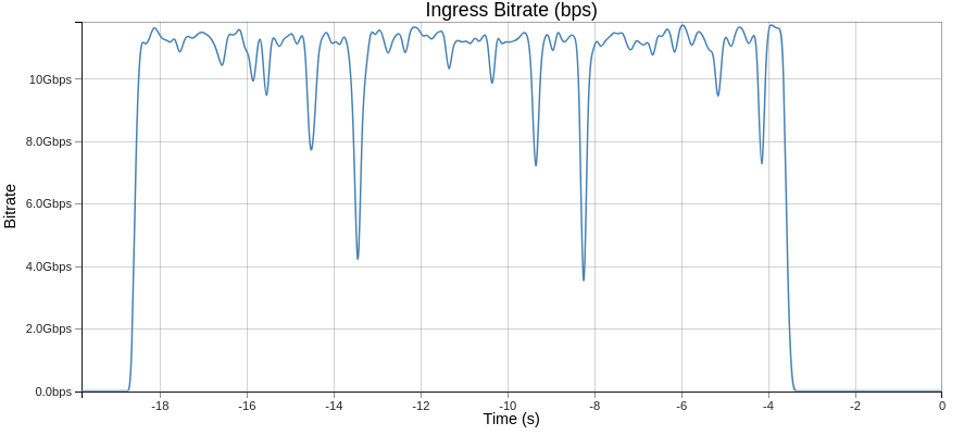
The throughput chart shows the effect of stalls (reduced bitrate), while the IPG chart shows their duration directly.

For statistical characterization, JitterTrap’s Flow Details view provides histograms of inter-packet gap and RTT distributions:

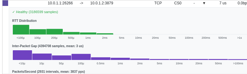
The IPG histogram reveals two distinct populations: the bulk of packets arrive with microsecond gaps (normal for saturated TCP), while the stalls appear as a long tail extending toward 100ms+. The mean IPG of 3μs confirms the baseline is healthy—the outliers from sender stalls are immediately visible as anomalies. This statistical view helps distinguish systematic sender problems from occasional glitches.

Network and Receiver Detection: TCP Signals

For the second and third diagnostic checks, JitterTrap’s TCP Window chart shows the advertised receive window for each flow over time, with event markers highlighting the exact moments problems occur:

Marker	Meaning	Diagnostic Value
⚠️ Zero Window	Receiver advertised zero window	Receiver problem confirmed
↻ Dup ACK	Duplicate acknowledgement	Possible packet loss
↩ Retransmit	Retransmitted segment	Network problem indicator
▼ ECE	ECN-Echo flag	Queue congestion (router signaled)
▲ CWR	Congestion Window Reduced	Sender responded to ECE

When a receiver can’t keep up, you’ll see the window collapse toward zero in the chart, followed by the ⚠️ marker. During recovery, the window gradually climbs back as the receiver drains its buffer.

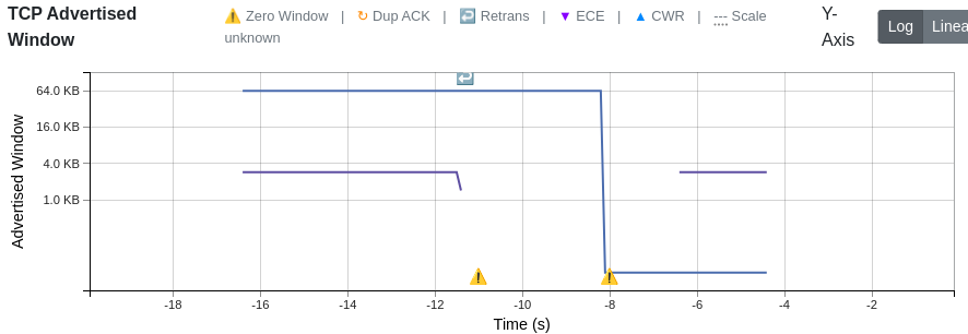
In this capture from a simulated receiver stall, the advertised window (blue line) drops sharply from 64KB to near-zero around t=-11s, triggering the first Zero Window marker (⚠️). The window recovers briefly, then drops again at t=-8s. Notice the Retrans marker (↩) appearing during recovery—this is TCP’s persist timer probing to check if the receiver has space again.

The TCP RTT chart complements this by showing round-trip time for each flow. Stable RTT with collapsing window = receiver problem. Rising RTT with retransmit markers = network congestion.

The Gap: From Observables to Diagnosis

JitterTrap currently shows you the signals—but you have to count the markers yourself and apply the thresholds manually:

Current State	What’s Needed
Shows zero-window markers (⚠️)	Count them per time window, compare to threshold
Shows retransmit markers (↩)	Count them per time window, compare to threshold
Shows window size over time	Compute derivative, detect negative trends
No diagnostic summary	“Sender” / “Receiver” / “Network” / “Healthy” status
No masking awareness	Warning when network issues mask receiver status

Potential Improvements

Based on this research, JitterTrap could add:

1. Threshold-based counting: Automatically count zero-window and retransmit events per 10-second window
2. Diagnostic summary: Surface a simple problem classification per flow
3. Window trend indicator: Show whether the window is shrinking, stable, or growing—catching receiver stress before zero-window events occur (this would address the 23% of receiver problems that never quite hit zero-window)
4. Masking effect warning: When network problems are detected, explicitly note that receiver status is unknown and re-testing is needed

---

What’s Next: The Jitter Cliff and Real-World Testing

This framework—zero-window for receiver, retransmits for network—works with 77-84% accuracy under controlled conditions. But during the experiments, I discovered something unexpected: a threshold where TCP behavior becomes chaotic.

When network jitter exceeds approximately 20% of the RTT, throughput doesn’t degrade gracefully—it collapses. And in this “chaos zone,” single measurements become unreliable. The coefficient of variation exceeds 100%.

Part 2 will explore:

• The jitter cliff: Why TCP collapses at high jitter, and what the RTO mechanism has to do with it
• BBR vs CUBIC: When to switch congestion control algorithms (spoiler: BBR provides 3-5x improvement in lossy environments)
• Real-world application: Applying this framework to Starlink and other challenging network conditions

---

Summary

The diagnostic framework:

• Inter-packet gaps exceeding application threshold (e.g., > 60ms for 30fps video) with healthy TCP signals → Sender problem
• Zero-window events > 5 in 10 seconds → Receiver problem (77% accuracy)
• Retransmits > 10 in 10 seconds → Network problem (84% accuracy)

The critical caveat:

• Network problems mask receiver problems
• If you detect a network problem, fix it first, then re-test

For JitterTrap:

• Surface zero-window counts in flow analysis
• Implement the decision tree in user-facing diagnostics
• Add explicit guidance about the masking effect

Limitations:

• All experiments were simulations using tc/netem for impairment injection—no production traffic or real-world captures were used for validation
• Thresholds are empirical heuristics that may need tuning for different environments
• Sender stalls are only detectable when stall duration exceeds RTT (the RTT ceiling limitation)
• 77-94% accuracy means we’ll miss some problems and occasionally misclassify others

This isn’t a perfect oracle. But it’s dramatically better than guessing, and it provides a systematic framework for diagnosis.

This research is part of Project Pathological Porcupines—an ongoing systematic exploration into the kinds of issues that delay-sensitive networking applications encounter, and how JitterTrap can help us understand these problems and improve our applications. Both the research and JitterTrap itself are works in progress.