The Jitter Cliff: When TCP Goes Chaotic
Part 2: Why throughput collapses and what to do about it
In Part 1, we used “video over TCP” as a stress test for TCP’s behavior—examining how zero-window events, retransmits, and the masking effect reveal what’s happening inside a struggling connection.
But during those experiments, I discovered TCP throughput degraded rapidly as jitter worsened. While I knew that packet loss would destroy TCP throughput, I hadn’t quite expected the jitter-induced cliff.
At a certain jitter threshold, throughput collapses so severely that measurements become unreliable. Single tests can vary by over 100%. This “chaos zone” makes diagnosis treacherous: the same network conditions can produce wildly different results depending on when you measure.
This post explores TCP’s behavior under jitter and loss, comparing CUBIC and BBR. It’s common knowledge that TCP is inappropriate for delay-sensitive streaming data, and this post will try to demonstrate how and why.
Experimental Setup
The findings in this post come from controlled experiments using Linux network namespaces with tc/netem to inject precise network impairments (delay, jitter, loss).
Why these constraints? We wanted to study a single TCP stream carrying streaming data—video, audio, or telemetry—where the application produces data at a relatively consistent rate rather than as fast as possible. This differs from bulk file transfers, where the goal is maximum throughput and applications use large buffers with TCP autotuning (up to 32 MB on Linux). By using a modest receive buffer (256 KB) and a fixed send rate (80 Mbps), we model a constrained streaming scenario where the jitter cliff behavior becomes visible. The absolute throughput numbers in this post reflect this setup; the ratios between algorithms and conditions are what generalize.
Key parameters:
| Parameter | Value | Notes |
|---|---|---|
| Target send rate | 10 MB/s (80 Mbps) | Sender paced at this rate |
| Receive buffer | 256 KB | Sized to avoid zero-window events |
| RTT range | 24-100ms | Controlled via netem delay |
| Jitter range | 0-24ms | Controlled via netem delay ... distribution |
| Loss range | 0-5% | Controlled via netem loss |
| Duration | 10 seconds per test | Multiple iterations for statistical validity |
| Topology | veth pairs | Between Linux network namespaces |
The receive buffer was set to 256 KB via SO_RCVBUF. Linux doubles this value internally for bookkeeping overhead (see socket(7))—verified by getsockopt() returning 512 KB. Packet capture analysis showed:
- Requested: 256 KB (
setsockopt) - Allocated: 512 KB (
getsockopt) - Maximum advertised window: 313 KB
- RTT: 50.2ms (from TCP timestamps)
This gives a theoretical maximum of 313 KB / 0.050s ≈ 50 Mbps. The measured baseline of ~42 Mbps is 85% of this theoretical maximum—the gap reflects TCP overhead from slow start, congestion window probing, and ACK timing. All figures in this post are relative to this ~42 Mbps baseline.
Why baseline throughput is ~42 Mbps, not 80 Mbps: TCP throughput is limited by the bandwidth-delay product (BDP)—the amount of data that can be “in flight” (sent but not yet acknowledged) at any moment. With 50ms RTT, the sender can only have ~50ms worth of data outstanding before it must wait for acknowledgments. Even in these benign conditions, throughput is significantly below the target rate of 80 Mbps.
The experiments compared CUBIC (Linux default) and BBR congestion control algorithms.
Results were obtained from more than 1500 experimental runs, sweeping the jitter, delay, loss and Congestion Control Algorithm parameters, using Linux kernel 6.12 with BBRv3.
The Jitter Cliff: RTT-Relative Collapse
A moderate amount of jitter (variation in packet delay) is inevitable on real networks. Routers queue packets, wireless links have variable latency (variable transmission rates due to variable modulation coding schemes), and congested paths add unpredictable delays. TCP is designed to handle this, within bounds.
This investigation is about learning where the boundaries are and what happens near them. Part 1 showed there is a rapid decay in throughput. Let’s characterise it: The cliff occurs when jitter reaches roughly 15-30% of the RTT, depending on the congestion control algorithm and conditions.
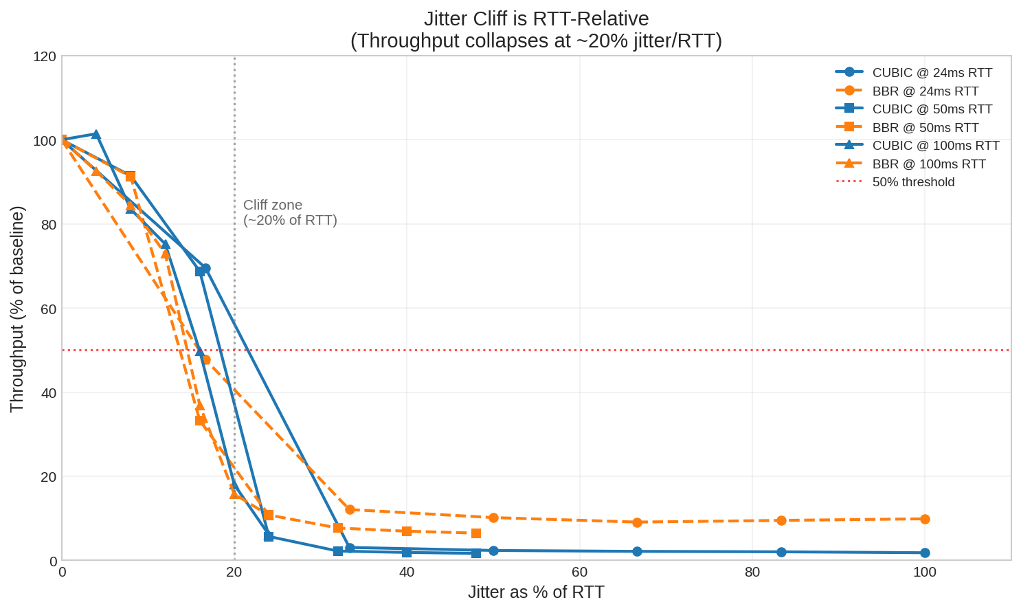
The plot shows throughput retention (percentage of maximum achievable throughput) versus jitter expressed as a percentage of RTT. Above 50% retention is functional; below is degraded or unusable.
| RTT | CUBIC Cliff | BBR Cliff | Notes |
|---|---|---|---|
| 24ms | ±8ms (33%) | ±4ms (17%) | BBR more sensitive at low RTT |
| 50ms | ±12ms (24%) | ±8ms (16%) | BBR collapses earlier |
| 100ms | ±16ms (16%) | ±16ms (16%) | Both similar at high RTT |
Notably, BBR’s cliff occurs earlier than CUBIC’s at lower RTTs. At 50ms RTT, BBR starts degrading at 16% jitter while CUBIC holds until 24%. BBR’s pacing model is more sensitive to timing disruptions from jitter, even though it handles packet loss better (as we’ll see later).
These thresholds matter because real-world networks operate in this range. Starlink, for example, has baseline jitter of ~7ms with ~27ms RTT—a 26% ratio, right at the CUBIC cliff. We’ll examine this in detail later.
The Counter-Intuitive Implication
This leads to a surprising conclusion: higher RTT means more jitter tolerance.
At ±12ms of jitter:
- 50ms RTT: CUBIC 2.4 Mbps, BBR 4.7 Mbps (collapsed—jitter is 24% of RTT)
- 100ms RTT: CUBIC 16 Mbps (functional—jitter is only 12% of RTT)
That’s nearly a 7x difference in CUBIC throughput for the same absolute jitter, despite the higher RTT.
This matters for network paths that include a satellite hop: the satellite segment may contribute more or less to the TCP throughput collapse than you might imagine. If the 20% rule holds, a geostationary satellite link with 600ms RTT could theoretically handle ±120ms of jitter while a 50ms LEO hop would collapse at ±10ms. (Note: GEO latencies were not simulated or tested—this is an extrapolation.)
The Chaos Zone: Why Single Measurements Lie
Near the jitter cliff, results become highly variable. Run the same test five times and you might get five dramatically different answers.
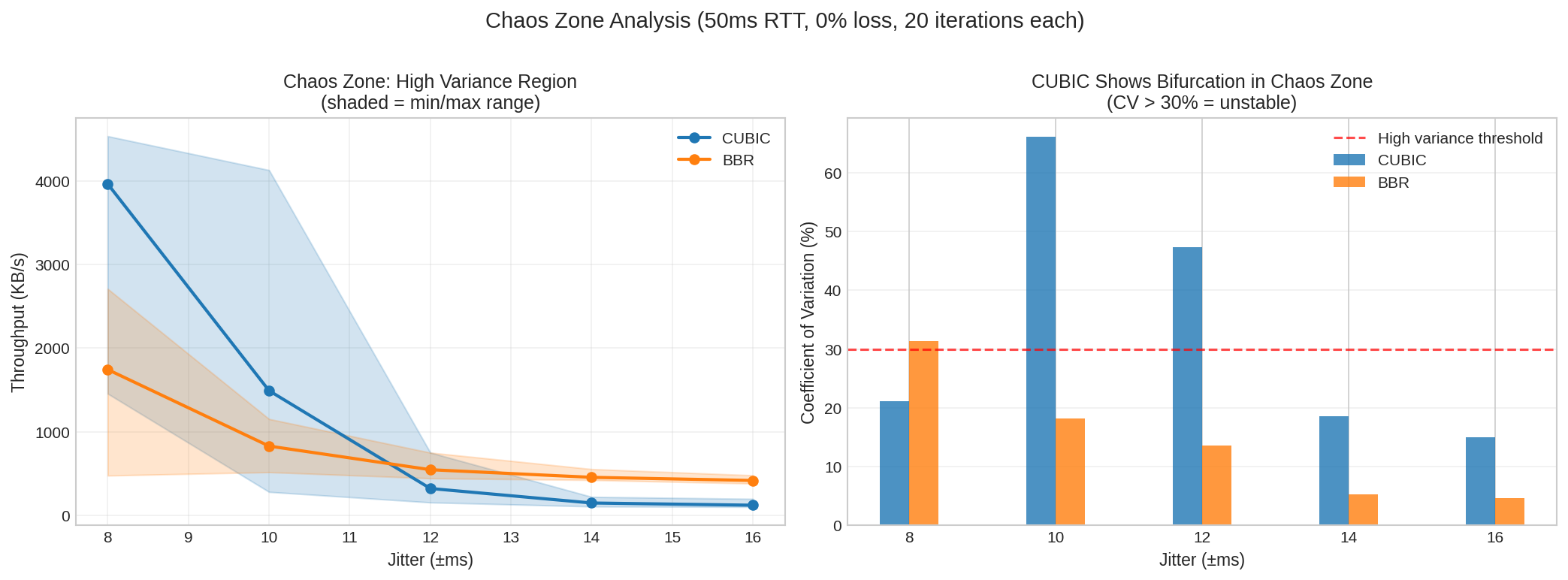
| Region | CUBIC CV | BBR CV | Interpretation |
|---|---|---|---|
| Below cliff | 1-5% | 1-5% | Stable, predictable |
| At cliff (chaos zone) | 21-66% | 14-31% | CUBIC unstable, BBR more predictable |
| Above cliff | 5-19% | 3-5% | Both collapsed, BBR still more stable |
In the chaos zone at 50ms RTT with 10ms jitter, CUBIC showed coefficient of variation up to 66%—meaning throughput varied wildly between runs. BBR’s CV stayed below 20% even in the worst conditions.
Practical implication: If your network operates near the jitter cliff (jitter 10-30% of RTT), don’t trust single measurements. Run at least five tests and look at the distribution.
Why CUBIC Becomes Unpredictable
What causes CUBIC’s high variance in the chaos zone? The data shows the pattern clearly, even if the mechanism is complex.
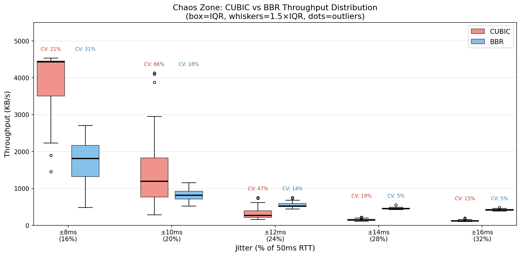
At 10ms jitter (20% of RTT):
| Algorithm | Range | Mean | CV |
|---|---|---|---|
| CUBIC | 2-33 Mbps | 12 Mbps | 66% |
| BBR | 4-9 Mbps | 7 Mbps | 18% |
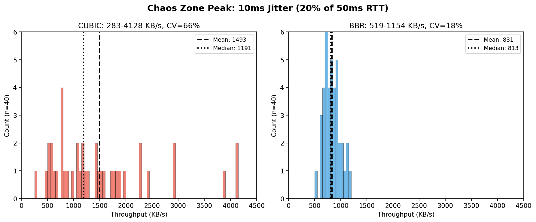
CUBIC’s distribution has a long right tail—occasional “lucky” runs achieved 3-4x the median throughput. BBR clusters tightly around its mean. This isn’t bimodal behavior; CUBIC seems to be highly sensitive to initial conditions while BBR remains consistent.
Packet capture analysis revealed the mechanism. The key metric is inter-packet gap—how long the sender waits between packets:
| Condition | CUBIC Gap | BBR Gap |
|---|---|---|
| Low jitter (stable) | ~0.5ms | ~0.5ms |
| High jitter (collapsed) | 5-8ms | 2-3ms |
When jitter crosses the threshold, CUBIC’s gap jumps 10-15x. BBR’s grows only 4-6x. Longer gaps mean lower throughput.
The hypothesis: High jitter causes spurious loss detection—packets arriving out of order or delayed beyond the retransmit timeout get mistaken for lost packets. Each “loss” triggers a cwnd reduction. But recovery is slow: during congestion avoidance, cwnd grows by roughly one segment per RTT. Above the threshold, reductions compound faster than recovery, and cwnd cascades toward its minimum. BBR survives better because its pacing-based approach doesn’t reduce sending rate aggressively on loss.
Caveat: We measured inter-packet gaps, not cwnd directly. This mechanism is plausible but not proven.
BBR vs CUBIC
Linux defaults to CUBIC for congestion control. BBR (Bottleneck Bandwidth and Round-trip propagation time) is an alternative developed by Google. The question everyone asks: which is better?
The answer: it depends on the amount of jitter and loss you expect on your path. For low amounts of jitter and loss, CUBIC still has a role to play.

The heatmap shows the BBR/CUBIC throughput ratio across different RTT and jitter combinations. Green means BBR is better, red means CUBIC is better, and yellow means they’re roughly equal.
When BBR Wins
| Condition | BBR Advantage |
|---|---|
| Jitter > 30% of RTT | 3-5x better |
| Post-cliff (both algorithms collapsed) | 3-5x better |
| Any significant packet loss | 2-17x better |
After the cliff, CUBIC flatlines at 0.7-0.9 Mbps while BBR maintains 3-5 Mbps. BBR degrades gracefully; CUBIC collapses sharply.
When CUBIC Wins (or Ties)
| Condition | Result |
|---|---|
| Jitter < 10% of RTT | Similar or CUBIC slightly better |
| Clean network, no loss | Similar performance |
The Surprising Middle Ground
In the chaos zone (jitter 10-30% of RTT), BBR can actually be worse than CUBIC in terms of mean throughput. At 50ms RTT with ±8ms jitter (16% of RTT):
- CUBIC: 29 Mbps mean (but CV = 21%)
- BBR: 14 Mbps mean (CV = 31%)
- BBR/CUBIC ratio: 0.49x
BBR achieves roughly half the throughput of CUBIC at this operating point. However, CUBIC’s higher mean masks significant run-to-run variance. In the worst part of the chaos zone (±10ms jitter), CUBIC’s CV reaches 66%—meaning some runs achieve good throughput while others collapse entirely.
This caught me off guard. BBR’s model-based approach sometimes makes suboptimal decisions in conditions where CUBIC’s loss-based reactions happen to work better. However, BBR’s lower throughput is predictably lower—and for video streaming, predictable throughput often matters more than maximum throughput.
Loss Tolerance: Where BBR Dominates
Jitter creates complexity for TCP, but packet loss is where CUBIC truly struggles.
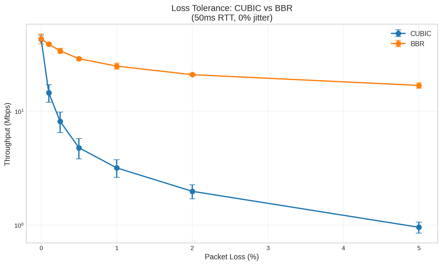
| Loss Rate | CUBIC | BBR | BBR Advantage |
|---|---|---|---|
| 0% | 43 Mbps | 43 Mbps | 1.0x |
| 0.1% | 14 Mbps | 39 Mbps | 2.8x |
| 0.25% | 8 Mbps | 34 Mbps | 4.2x |
| 0.5% | 5 Mbps | 29 Mbps | 6.1x |
| 1% | 3 Mbps | 25 Mbps | 7.8x |
| 2% | 2 Mbps | 21 Mbps | 10.6x |
| 5% | 1 Mbps | 17 Mbps | 17.6x |
(Tested at 50ms RTT, 0% jitter, 5 iterations per condition)
Even 0.1% packet loss—one packet in a thousand—causes CUBIC throughput to drop by 67%. BBR maintains 91% efficiency at the same loss rate.
At 5% loss, the difference is staggering: BBR provides 17.6x the throughput of CUBIC.
Why the Asymmetry?
CUBIC interprets every lost packet as a congestion signal and aggressively backs off. This is appropriate when loss is caused by buffer overflow—it means the network is genuinely oversaturated.
But loss can have other causes: wireless interference, cable faults, router bugs, or even ECN-incapable middleboxes dropping marked packets. In these cases, backing off doesn’t help—the path capacity hasn’t changed, just some packets got corrupted.
BBR uses a model-based pacing approach. It estimates the bottleneck bandwidth and RTT independently of loss, and paces packets accordingly. Random loss doesn’t cause BBR to dramatically reduce its sending rate.
Recommendation
On any network with adverse jitter or packet loss, use BBR. The advantage is significant.
Real-World Application: Starlink
The experiments so far used synthetic conditions. How do these findings apply to real networks? Starlink provides a good test case—it has measurable jitter, occasional packet loss, and millions of users trying to stream video over it.
Realistic Starlink Characteristics
Based on published measurements:
| Metric | Typical Range | Source |
|---|---|---|
| RTT | 25.7ms median (US), 30-80ms range | Starlink official, APNIC |
| Jitter | 6.7ms average, 30-50ms at handover | APNIC |
| Packet Loss | 0.13% baseline, ~1% overall | WirelessMoves, APNIC |
| Handover | Every 15 seconds | APNIC |
Critically, Starlink’s loss is not congestion-related—it’s caused by satellite handovers and radio impairments. CUBIC’s loss-based congestion control misinterprets these as congestion signals, causing unnecessary throughput reduction.
Now we can connect these characteristics to the jitter cliff thresholds from earlier:
| Profile | Jitter | RTT | Jitter/RTT | Cliff Zone |
|---|---|---|---|---|
| Baseline | ±7ms | 27ms | 26% | At CUBIC cliff |
| Handover | ±40ms | 60ms | 67% | Past both cliffs |
| Degraded | ±15ms | 80ms | 19% | Chaos zone |
Starlink’s baseline operation—not degraded, not during handover, just normal—sits right at the CUBIC cliff threshold. This explains why TCP performance over Starlink is so sensitive to congestion control algorithm choice.
Experimental Results
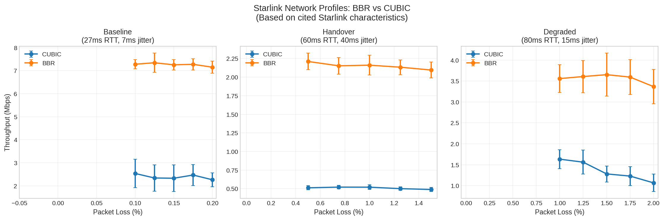
| Profile | RTT | Jitter | Loss | CUBIC | BBR | BBR Advantage |
|---|---|---|---|---|---|---|
| Baseline | 27ms | ±7ms | 0.125% | 2.3 Mbps | 7.3 Mbps | 3.1x |
| Handover | 60ms | ±40ms | 1.0% | 0.5 Mbps | 2.2 Mbps | 4.2x |
| Degraded | 80ms | ±15ms | 1.5% | 1.3 Mbps | 3.7 Mbps | 2.9x |
(200 iterations per profile, parameters matched to cited Starlink characteristics)
Even at baseline conditions with only 0.125% loss, BBR provides 3.1x the throughput of CUBIC.
A note on absolute vs. relative throughput: The absolute Mbps values above reflect our constrained test setup (256 KB buffer, single stream). Real-world Starlink achieves higher absolute throughput because applications use larger buffers and speed tests use multiple parallel connections. However, the ratios we measured match real-world observations remarkably well.
Real-World Validation
Independent testing on actual Starlink connections confirms the pattern we observed in simulation:
| Source | CUBIC | BBR | BBR Advantage |
|---|---|---|---|
| Our simulation | 2.3 Mbps | 7.3 Mbps | 3.1x |
| WirelessMoves (2023) | ~20 Mbps | >100 Mbps | ~5x |
The WirelessMoves testing used single-connection iperf3 tests over real Starlink hardware. Despite the 10x difference in absolute throughput (due to larger buffers and different conditions), the BBR advantage ratio is consistent: 3-5x better than CUBIC.
This also explains why Starlink users don’t universally complain about poor TCP performance:
-
Speed tests use multiple parallel connections. Speedtest.net and similar tools aggregate many TCP streams, masking single-connection limitations. A user might see “150 Mbps” on Speedtest while a single video stream struggles at 20 Mbps with CUBIC.
-
Many major services use BBR. Google, Netflix, and Cloudflare have deployed BBR on their servers. Users streaming from these services get BBR’s benefits without changing anything on their end.
-
Adaptive bitrate masks the problem. Video services like YouTube and Netflix adjust quality based on available throughput. Users see “480p” instead of “buffering,” which feels like a content choice rather than a network failure.
Video Quality Mapping
What does this mean for actual video quality?
| Condition | With CUBIC | With BBR | Recommendation |
|---|---|---|---|
| Baseline (2.3 vs 7.3 Mbps) | 360p choppy | 720p smooth | BBR strongly recommended |
| Handover (0.5 vs 2.2 Mbps) | Unusable | 360p barely | BBR + buffer for handovers |
| Degraded (1.3 vs 3.7 Mbps) | 360p choppy | 480p usable | BBR essential |
Video quality estimates assume ~2.5 Mbps for 480p, ~5 Mbps for 720p (H.264). These represent relative performance differences between algorithms under simulated Starlink conditions.
The Handover Problem
Starlink satellites hand off every 15 seconds. During handover (per APNIC measurements):
- RTT spikes by 30-50ms (e.g., 30ms → 80ms)
- Jitter increases significantly
- Packet loss spikes occur
These are brief disruptions, not 15-second outages. Video applications need enough buffer to absorb the throughput dip during handover—likely a few seconds, not 15.
Practical Recommendations
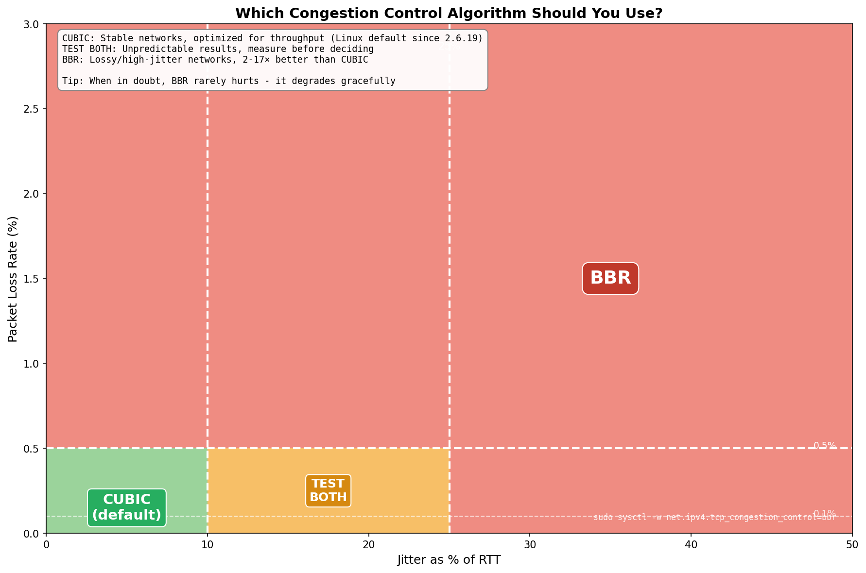
Decision Guide
- Stable networks (jitter < 10% of RTT, loss < 0.1%): Use CUBIC (Linux default)
- Moderate jitter (10-30% of RTT): Test both algorithms—results vary
- High jitter (> 30% of RTT): Use BBR
- Any significant packet loss (> 0.1%): Use BBR
- Satellite links (Starlink, LEO, GEO): Use BBR
How to Switch Congestion Control
# Enable BBR (requires root, kernel 4.9+)
sudo modprobe tcp_bbr
sudo sysctl -w net.ipv4.tcp_congestion_control=bbr
To make permanent, add tcp_bbr to /etc/modules-load.d/bbr.conf and net.ipv4.tcp_congestion_control=bbr to /etc/sysctl.conf.
Implications for JitterTrap
This investigative work was done to support JitterTrap. When users report video stuttering or unexplained throughput problems, the tool needs to help them understand why—not just show that something is wrong. The jitter cliff and chaos zone findings directly inform what JitterTrap should measure and how it should present that information.
Planned improvements based on this work:
- Jitter/RTT ratio indicator: Show whether the network is below, at, or above the cliff threshold
- Chaos zone warning: Alert when measurements may be unreliable (jitter 10-30% of RTT)
- Congestion control guidance: Recommend BBR vs CUBIC based on observed conditions
- Stability indicator: Display coefficient of variation to distinguish consistent problems from chaotic ones
The Bigger Picture
The jitter cliff is a real problem for video over TCP. Throughput can collapse by 90% or more, and near the cliff, behavior becomes unpredictable. But understanding why this happens points to a deeper issue.
TCP’s flow control relies on back-pressure: when the network is impaired, TCP slows down and signals the sender to wait. This works for file transfers, database queries, or web requests—applications that can pause. But video can’t pause:
-
Applications that cannot slow down: A live video encoder produces frames at a fixed rate regardless of network conditions. When TCP’s send buffer fills, frames queue up, latency grows unboundedly, and eventually data drops catastrophically. TCP signals back-pressure, but the encoder has no mechanism to respond—it can’t “skip this frame” or “reduce bitrate” based on socket buffer state.
-
Disconnected back-pressure: Consider UDP video inside a TCP VPN tunnel. When TCP throughput drops—due to the jitter cliff, loss, or BDP limits—the video source keeps sending at its configured rate while the tunnel delivers at a fraction of that. Latency climbs as data queues. TCP retransmits packets the receiver may no longer care about. The back-pressure never reaches the encoder.
The jitter cliff isn’t a bug in TCP—it’s TCP doing what it was designed to do. The failure is architectural: TCP guarantees “deliver everything, in order, eventually,” but video needs “deliver what you can now, drop what’s stale, and tell me to adapt.”
Summary
- The jitter cliff: Throughput collapses when jitter exceeds roughly 15-30% of RTT. Higher RTT = more tolerance.
- The chaos zone: Near the cliff, CUBIC varies 21-66%; BBR stays at 14-31%. Don’t trust single tests.
- BBR vs CUBIC: BBR wins under loss (up to 17.6x better) and post-cliff. CUBIC can win in the chaos zone but is less predictable.
- Practical: Use BBR on lossy or satellite networks; CUBIC on stable networks; test both near the cliff.
- Limitations: Lab simulation (1,500+ runs, Linux 6.12/BBRv3) validated against real-world Starlink measurements showing consistent ratios.
What’s Next
Part 3 will explore SRT (Secure Reliable Transport)—a protocol designed specifically for live video that borrows from TCP but fixes what makes TCP unsuitable:
- Bounded latency: SRT enforces a maximum latency; packets that arrive too late are dropped, not delivered
- Sender feedback: The receiver reports packet loss and timing back to the sender, enabling adaptive bitrate
- Selective retransmission: Only retransmit packets that can still arrive in time
- Application-layer control: The video encoder can respond to network conditions
SRT asks the right question: “What can I deliver within this latency budget?” rather than TCP’s “How do I eventually deliver everything?”
This research is part of Project Pathological Porcupines—an ongoing systematic exploration into the kinds of issues that delay-sensitive networking applications encounter, and how JitterTrap can help us understand these problems and improve our applications. Both the research and JitterTrap itself are works in progress.