JitterTrap: Baby steps in DSP

This is the story of my first expensive lesson in Digital Signal Processing. It is about JitterTrap, the free software that powers BufferUpr.

The premise of BufferUpr is to combine commodity hardware with open source software to create a product that can measure data stream delays of 1-100 milliseconds. This is the range of delay that most multimedia developers and consumers are concerned with.

To measure the delay, we count the packets and bytes as they fly past and look for changes in throughput. My naive logic was that if we look at consecutive intervals of 1ms, we'll be able to measure the throughput over that interval, plot it and show any variation in throughput.

This seemed like a very simple task, except that I had no previous experience in Digital Signal Processing and didn't see why that would be relevant.

Technical Problem

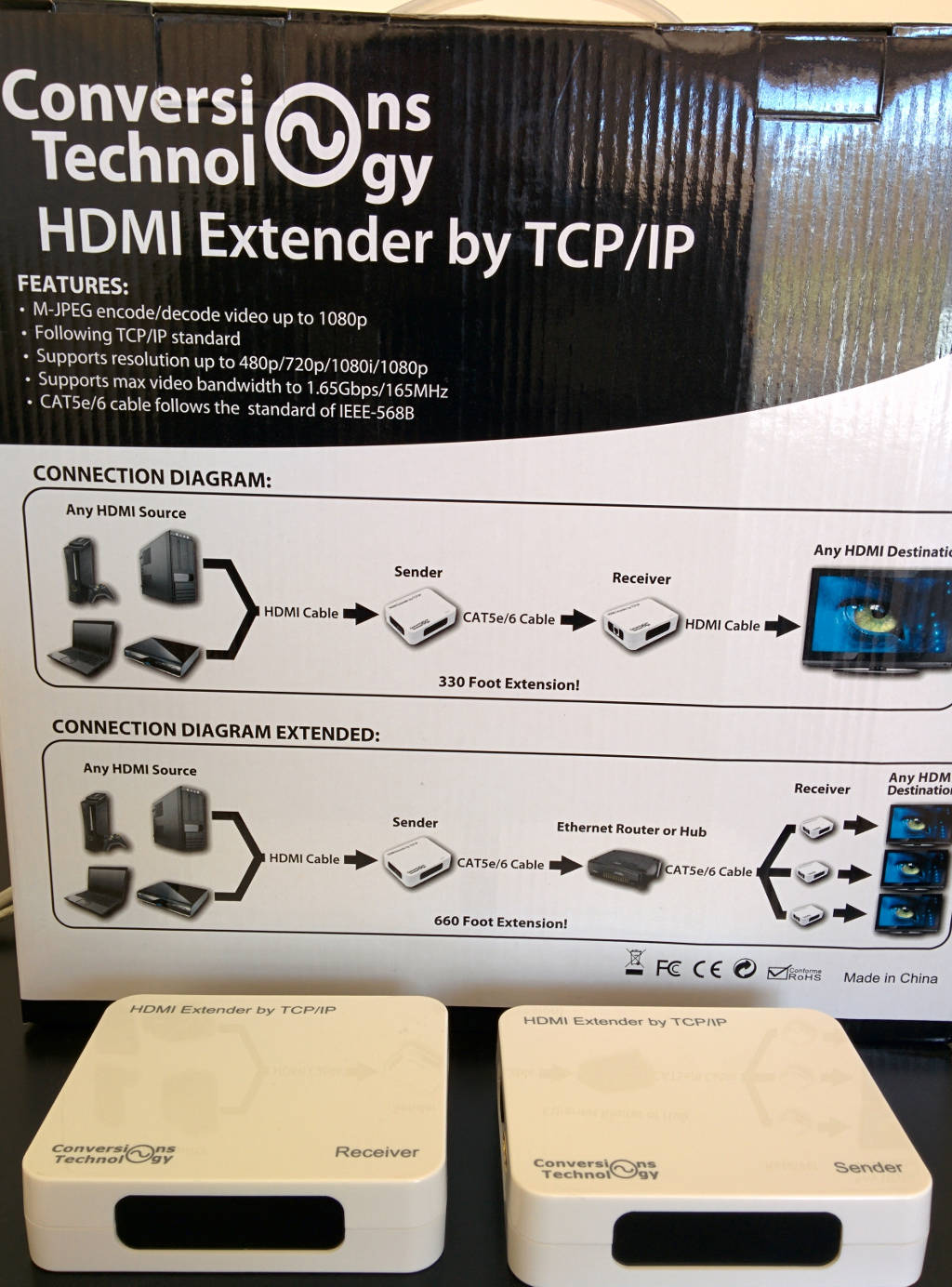
Shortly after I had a first working prototype I ordered some streaming hardware to test my new creation with - an "HDMI Extender by TCP/IP".

It takes an HDMI video input, encodes & sends it over IP. The receiver decodes it and outputs HDMI.

Using JitterTrap, I saw unexpected low frequency variations in the measured/plotted packet rates. Here's a still screen grab from the video:

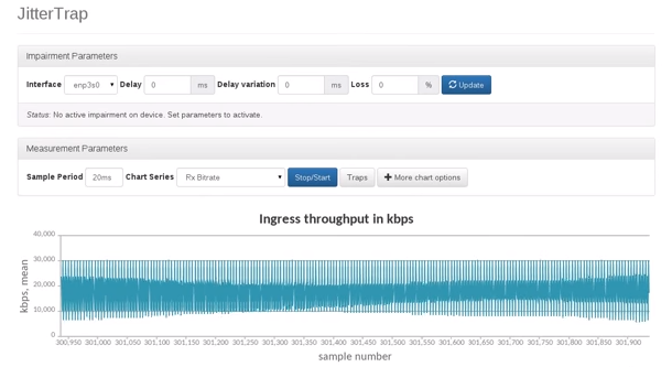
I expected the stream to have a consistent high packet rate, but the low frequency variation in packet rate changes, depending on the length of the intervals on the chart. That makes the measurements much less usable than I intended.

As I've been learning, this could be a symptom of aliasing, or moiré patterns, as several people have pointed out to me.

DSP101

(for people who don't know what side of the soldering iron to hold)

The Scientist and Engineer's Guide to Digital Signal Processing explains aliasing as a low frequency misrepresentation of real signal and a consequence of incorrect sampling.

From the Nyquist/Shannon sampling theory, we know that the sample rate must be greater than 2 x the highest frequency in the signal in order to have enough information to reconstruct the signal perfectly and avoid aliasing.

Let's consider the packet rates of gigabit Ethernet and the sample rate of JitterTrap...

In IP over gigabit Ethernet networks, minimum-sized packets can arrive every 640ns. The maximum rate for minimum sized packets is therefore 1/640ns - roughly 1.5 Million packets per second (1.5Mpps).

Here's the calculation:

Gigabit Ethernet has a minimum receive-side inter-packet gap (IPG) of 64 bit times. In other words: 8 octets, at 1 million bits per second, is 64 nanoseconds.

After the IPG, before the Ethernet headers for the next packet, comes the Preamble of 7 octets and Start Frame Delimiter of 1 octet.

We have:

   | IPG      | Preamble | SFD     | Ethernet Headers + Payload + FCS |
=  | 8 octets | 7 octets | 1 octet | 64 octets                        |
=  |                     80 octets                                    |


80 octets @ GbE = 80 * 8 bit times
                = 640ns
                = 64ns IPG + 576ns Packet

We can also think of this in terms of a square wave where the duty cycle is:

D = T / P
  = 576 / 640
  = 90%

Now we know we have something that we can think of as a cycle with length 640ns, or a frequency of 1/640ns.

F = 1/640ns
  = 1/0.000000640s
  = 1562500Hz
  ≈ 1.5MHz

If the maximum packet rate is 1.5Mhz, the packet counter can theoretically jump from zero to 1.5M over two consecutive 1s intervals, therefore the sampled "signal" has a maximum frequency (and bandwidth) of 1.5MHz.

JitterTrap (in it's flawed 2015 implementation) samples the Ethernet frame counter to obtain a measurement of the packets received over a specific sample interval. The sample interval is currently 1ms, i.e., the sample rate is 1kHz.

All together now, in the voice of Adam Savage: "well, there's yer problem!".

Well, is it really that simple?

If the packet rate is high, lets say 50kpps, but fairly constant, we can still get a nice straight line at the expected value. Why is that? In what way does it not work?

Lessons from video

Video has a very familiar example of aliasing called the wagon-wheel effect. Here's a demo from Jack Schaedler's excellent primer on DSP.

You'll see that for very low sample rates, the snapshots on the right move counter-clockwise. For moderately high sample rates, the snapshots rotate clockwise, but slower than the wagon wheel.

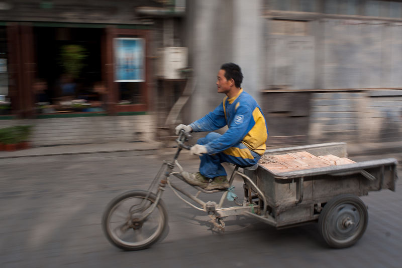
That's still not the complete story. What we saw above is a generated image. In a sampled image, like a photo or a single frame in the video sequence, we also see motion blur due to the sample interval being relatively long.

An image sensor consists of a grid of photosites that collect electric charge as photons strike them. The more photons, the more charge.

Therefore the camera is taking a sample of the visible light spectrum...

• over a specific time interval.

• in two spatial dimensions

The time interval measured by the still frame is MUCH longer than the time for one wavelength of visible light to reach the sensor.

In the image above, the camera shutter was open for 1/30s (33.33ms). However, visible light has wavelengths in the range from 390–700nm, which corresponds to frequencies of 430–770 THz.

[I think it's safe to say that sampling at twice the frequency of the visible light spectrum is probably not an option, though the has been some interesting developments with capturing ultra short pulses of light in so-called Femto Photography.]

If all modern digital photography suffers from aliasing, what does that mean? Can we relate the Nyquist-Shannon theory to the blurry photo to obtain a better understanding?

I think what happens is a smearing of the signal in the time domain. The energy is spread out over the frequency bands that can be recorded using this sampling mechanism, but the total energy carried by the photons remains the same as if we were able to record each photon individually.

Is this why we recording the wavelength (or frequency) of light is such a challenge? Most common sensors infer frequency information from a Bayer patterned filter. Only Foveon sensors make use of the absorbtion properties (where higher frequencies have lower penetration into the silicon) to discretize the frequency of the photon.

Now, think about the two spatial dimensions. The light is collected over an area. Leaving aside all the intricacies of photosites and point spread functions, we can clearly see from motion blur that there is a range of positions where we saw the wheel.

If we know how long the interval is that we saw it, and combine that with the measured distance it moved during that time, we can calculate the speed. [Granted, maybe we can't measure speed from my mediocre panning shot above, but in theory it's possible.]

Motion blur in the image above is like a moving average with a direction in the spatial domain. The pixels that show the motion blur contains a mixture of light that originated from points that are adjacent at any instant in time.

Let's add flash photography to the model.

With flash photography, the duration of the illumination from the flash is typically much shorter than the total exposure time and much brighter than the ambient light. This localises the energy of the signal in time and therefore reduces the motion-induced blur in the spatial domain.

If the value of each photosite represents an average of the luminosity of a stationary point in the focused image over a period of time, then the detail that we perceive are the changes in the average energy over distance. In other words, it's the transitions between low and high brightness that provide texture and contrast.

What does photography and videography have to do with packet counters?

For JitterTrap, just as with images, we are interested in the average over a long period, as well as patterns and irregularities in the variation of the average.

The important observation is that each photosite acts as a photon counter of sorts - counting each photon and storing the accumulated count.

What the network packet counter is doing is the same - recording each received packet and storing the accumulated count.

In each case we can read the counter after an interval of time has passed and obtain an average of the signal. This kind of integration and averaging, where each sample has equal weight, is called a boxcar filter.

We can also say that the filter uses a rectangular window function. This is a simple kind of low-pass filter and it has some undesirable properties in the frequency representation due to the discontinuities of the windowing function.

The sharp transitions between 10000 and 30000 in the JitterTrap screenshot above is due to the rectangular windowing function. The low-frequency pattern is a moiré pattern, which is also a problem in digital cameras.

Most digital cameras use an optical anti-alias filter to artificially blur the image before it reaches the sensor to prevent this moiré pattern. This also means that the sensor is not capturing at the highest possible spatial frequency.

So it seems that there is a trade-off to make here. A smoother plot, without the moiré pattern is certainly possible, but necessarily also blows away some of the high frequency transients.

What would Wireshark do?

What if we had a precise and accurate timestamp for every packet and used that to plot our packets, like what Wireshark does?

Well, let's see...

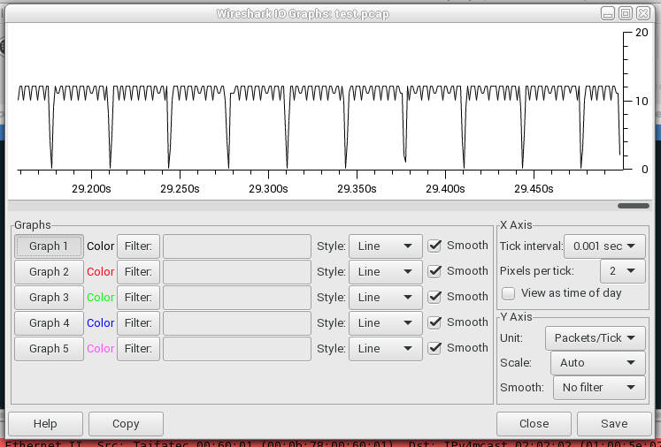
And here's another screengrab from the jittertrap video at the 44 second mark.

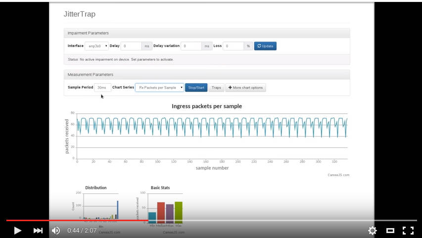
The second image is quite hard to read, which is lucky, because the scales on the axes are wrong, but if you close one eye and squint with the other, we can pretend that the two graphs have some resemblences.

Note that the depths of the valleys change in both the JitterTrap and Wireshark plots.

Why sample? Why not do what Wireshark does?

Initially the concern was that packet capture at high rates is too CPU intensive. My intention is that JitterTrap should run well on small embedded devices and from the number of projects like PF_RING, PFQ that specialise in efficient packet capture, it seemed like this is hard to do well.

With Linux features like packet_mmap and NAPI, it might be good enough. I have done some tests and it looks OK. I should probably post my measurements...

In any case, I'm still debating whether it's worth persuing this path. [Comments welcome!]

Why sample at 1ms intervals?

For applications running on a general purpose CPU and operating system like Linux with good scheduling and good drivers, the mean error between desired and actual scheduled wake-up time can be anywhere between 20us and 150us... with a HUGE standard deviation.

These non-deterministic delays are a challenge that imposes certain limits on the accuracy and precision of measurements obtained through periodic scheduling.

Common solutions, in order of increasing determinism & cost and decreasing delay & jitter are:

• to work really hard to improve the software on a specific system configuration.

• to use a "real-time" operating system with tighter scheduling guarantees. This is basically the same thing as above: throw away everything that you don't need, determine the priorities of the things you keep, and pray that the remaining black boxes (like firmware) don't screw anything up.

• use a dedicated microcontroller that does nothing but your real-time IO task.

• use an FPGA.

JitterTrap is intended to run on Linux. My hope is that it becomes a familiar tool and a recognisable contribution to the community.

There are practical reasons that make Linux a good choice, besides development cost. Linux already has excellent network emulation capabilities that has been studied academically:

• Measuring Accuracy and Performance of Network Emulators by Robert Lübke, Peter Büschel, Daniel Schuster and Alexander Schill, published in Communications and Networking (BlackSeaCom), 2014 IEEE International Black Sea Conference on.  《cached here》

• A Comparative Study of Network Link Emulators by Lucas Nussbaum and Olivier Richard  《cached here》

• Network Emulation with NetEm by Stephen Hemminger  《cached here》

Conclusion

This is quite a long blog post and unfortunately it still isn't entirely convincing that the JitterTrap graphs and measurements are correct and reliable.

Hopefully it's clear that time-frequency analysis entails some unavoidable compromises and trade-offs, but is nevertheless quite useful and interesting.

With this background rambling of a DSP novice out of the way, the bulk of the writing for the past two months of study is still to come. I've been analysing some packet traces using SciPy and will provide more pictures and numbers (with less rambling) soon.

Discussion, comments and corrections are appreciated. Please send them to acooks@rationali.st

Thanks

Thanks to Justin Schoeman and Edwin Peer for corrections and feedback on previous drafts. All remaining errors are my own fault.

Thanks to Walter Smuts, Frans van den Bergh and Tom Egling for inspiring me to learn more about signal processing.